In our previous blog post, we discussed merits of building a machine learning algorithm to predict the outcome of March Madness. Now, it’s time to dive into the technical aspects of building a model. In this post we’ll provide a general framework and examples / guidance on executing these steps.
How to build your March Madness ML Model:
- Data collection: Obviously, the most important thing we need to do any sort of modeling is data. There is an extreme wealth of data available to you across the internet. More doesn’t always mean better when building a model, and the more data you decide to include, the more work that will be involved in the next step so keep that in mind . See below for in depth guidance on this topic.
- Feature engineering: This is the step where you will probably spend most of your time (or at least it should be if you want your model to do well). After you gather data, you need to transform that data into features that can be used as inputs to your model. This step is known as feature engineering, and involves techniques such as feature extraction, normalization / scaling, binning, etc. For example, a feature could be the difference in scoring average between two teams, or the difference in strength of schedule.
- Model training: The next step is to train the model on the data. To do this, you take your data and split it into a training, test, and validation data sets. The purpose of each dataset and guidance on creating them is discussed below. Once your data is split, you choose an algorithm that you will use to fit your ML model to the data, so that it can make predictions about the outcome of each game in the tournament.
- Model evaluation: After the model has been trained, the next step is to evaluate its performance. This can be done by comparing the model’s predictions to the actual outcomes of the games in the validation set. Common metrics for evaluating the performance of a predictive model include accuracy, precision, recall, and F1 score.
- Model Predictions for current season: Once you are satisfied, to “deploy” your model, run your predictions and use this information to fill out your bracket.
Data Collection
There is a wealth of data available. It makes the most sense to use the Kaggle datasets provided each year since that eliminates a lot of the data collection. Augmenting this data might be helpful, and some things that might be worth exploring and including in your model include: ELO Ratings, Massey Ratings, and Upset statistics.
In case you are unfamiliar with it, ELO ratings originated from the game of chess but have permeated into sports, competitive gaming etc. It was invented by Arpad Elo, a Hungarian-American physics professor, as a better chess-rating system over what existed prior. The simple approach makes it easy to generalize and apply to many other competitions. In essence, you start the season with each team having the same score. As games are played, the winning team takes points from the losing team and scores are adjusted. If a team beats another team with a much higher rating, they will take more points; if instead their opponent had a lower rating, they would take fewer points. The difference between the ELO ratings of two teams determines is used to predict the outcome of matches.
Some of the data you would expect to find the Kaggle datasets or through other means include:
Team statistics: Team-level metrics that provide a general sense of how a team has performed throughout the season would be stats like
- Win-loss record
- Points scored
- Points allowed
- Tournament seed
- Strength of schedule
Player statistics: There is no “I” in team but the same could be said about the presence of wisdom if one chose to ignore the individual players contribution to their teams performance. Stats in this category include things like:
- Field goals (2-pointers) scored
- Field goal attempts
- Three-pointers scored
- Three-pointer attempts
- Rebounds,
- Assists
Feature Engineering and Selection
Feature Engineering is the process of transforming the data you collected into inputs for your model. These steps will be specific to the data you collected. For instance if you are using the sample Kaggle datasets from the past, you’ll have a data set with the seeds of the winning and losing team in each game as well as their respective scores for every season since 1985. Instead of leaving them in their raw form, consider calculating the difference between the metrics of the winning team and losing team. For example, instead of having data that looks like this:
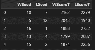
You would take Win seed column and subtract the loss seed column:
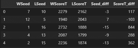
Using differentials instead of raw values helps us normalize our data and can remove some of the noise, making it easier to compare teams and generalize features across the seasons. For instance, if there was a rule change that imposed a faster shot clock, you’d expect to see an uptick in the number of points scored in each game compared to prior seasons. I’m not saying that happened, but if it did, using differentials allows us to ignore the “noise” introduced by the changing pace of the game and compare more meaningful stats.
It is important to understand the data you collect and what each feature you ultimately feed into your model represents, otherwise you may inadvertently end up hindering your model in making accurate predictions instead of helping it.
During your data collection, you will likely come across stats such as Player Efficiency Rating (PER), Team Offensive Rating, and Team Defensive Rating. Knowing how these features are calculated is useful because it can help safeguard against introducing multi-collinearity which, in layman’s terms, refers to a situation where two or more predictor variables are highly related to each other, and thus contain redundant information (selecting certain algorithms will also make our model less sensitive to this which we will get into soon).
Player Efficiency Rating (PER) is a metric that attempts to quantify a basketball player’s overall effectiveness and efficiency on the court. It was developed by John Hollinger, a former ESPN analyst, and is widely used by basketball analysts and statisticians.
The formula for calculating PER is quite complex, but it essentially takes into account a variety of offensive and defensive statistics, including points scored, rebounds, assists, steals, blocks, and more, and normalizes them based on the number of minutes played and the pace of the game. The formula also accounts for various in-game variables, such as the number of possessions and the shooting efficiency of the player’s team. The end result is a single number that represents a player’s overall contribution to their team’s success, with higher numbers indicating better performance. The average PER across the league is set to 15.00, and the league’s best players generally have a PER in the range of 25 to 30.
If you were focused on modeling player performance and used some of the more common / obvious metrics like points scored, rebounds, etc. and also included the PER for a player, you would be including redundant information and introducing multicollinearity which can have varying impact on your models performance.
Model Selection
There are many types of models that can be used to predict the outcome of the March Madness tournament. As mentioned above, we want our model to be able to capture non-linear relationships. Some of the many models capable of this include Neural Networks, SVMs, Decision Trees & Random Forests, and Gradient Boosting.
Decision Tree
A decision tree is a tree-based model that makes predictions by recursively partitioning the data into smaller and smaller subgroups based on the feature that best splits the data.
Decision trees are simple and easy to understand which is great when you need to provide information as to how your model made the decision it did. That doesn’t apply here but it is good to keep in mind.
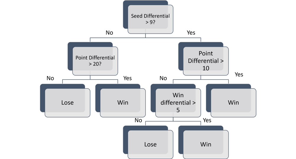
At each node in the tree, the algorithm makes a decision based on the values of the features, and the tree ultimately outputs a prediction for each sample in the data.
Decision trees can be prone to overfitting, especially when the tree is deep and complex. For this reason, it is wise to use a Random Forest model or Gradient Boosting.
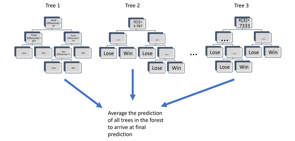
Random forests are an extension of decision trees, where multiple decision trees are trained on random subsets of the data and the prediction of the random forest is the average of the predictions made by each tree. This averaging of the predictions helps to reduce the variance in the predictions, making random forests well-suited for handling high variance in variables. Bootstrapping (random sampling of data with replacement) and the use of different subsets of data and predictor variables for training the various decision trees help prevent overfitting. Other regularization techniques to use with the decision trees are limiting the maximum depth a tree can have, the maximum number of leaf nodes, the maximum number of features that are evaluated for decision nodes.
Gradient boosting is an iterative algorithm that combines multiple simple models, such as decision trees, to create a more powerful and accurate model. The algorithm works by training each simple model on the errors made by the previous model, with the goal of reducing the error with each iteration. Gradient boosting helps prevent overfitting by building the models in a step-by-step fashion, to create a final ensemble of models that is well-balanced, and is not overly complex or fitting to noise in the data. It also uses regularization, which adds a penalty term to the loss function used to fit the models in order to discourage the models from becoming too complex or fitting too closely to the training data. This helps generalize models so that they can make more accurate predictions on new data.
Model Training and Evaluation
To build your model, you need to split the available data into two or more sets so that you can evaluate the performance of the model on new, unseen data and to avoid overfitting.
There are a couple of ways to split data:
- Train-test split: Data is divided into a training set and a testing set. The training set is used to train the model, while the testing set is used to evaluate its performance. Typically, the testing set contains around 20% to 30% of the available data, with the remaining data used for training.
- Cross-validation: Cross-validation involves dividing the training data into k folds, where each fold is used as a validation set once and the remaining data is used as a training set. The performance of the model is then averaged over the k folds. Cross-validation can be used to evaluate the performance of the model more accurately, as it uses all available data for training and testing. The picture below taken and edited slightly from scikit-learn illustrates the above 2 methods.
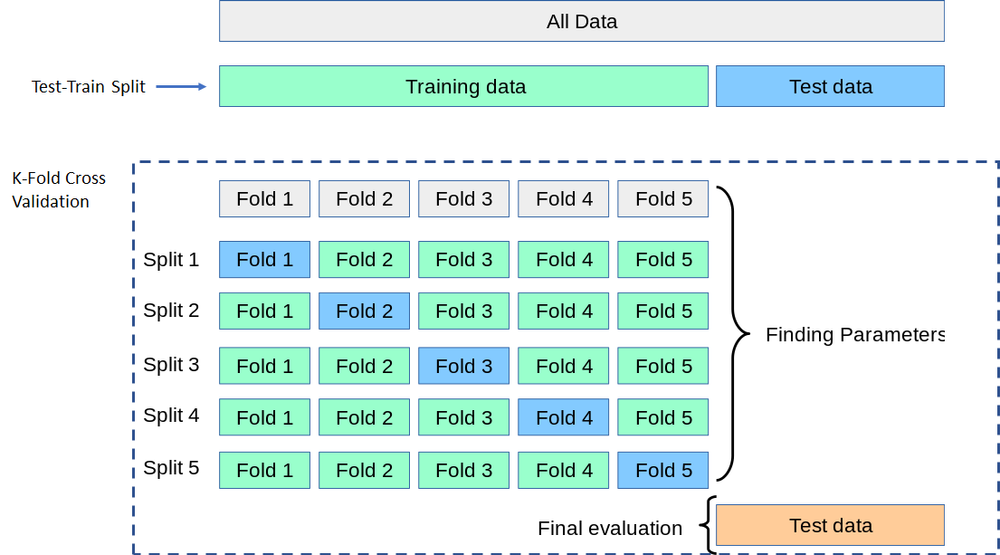
- Time-based split: In some cases, the data is time-dependent, such as in the case of stock prices, weather data, or tournaments in sports (why we are here!). In such cases, it is common to use a time-based split, where the data is split into a training set containing data from the earlier time period, and a testing set containing data from the later time period. For March Madness specifically, it makes sense to train on the regular season and test on the post season since the ultimate goal of our model is to predict that.
Beyond dividing your dataset up into a test and train dataset, you’ll want to spend some time thinking through some of the parameters and hyperparameters.
Once the data has been split, the model’s hyperparameters can be tuned to add more structure to the training and optimize its performance on the testing set. Hyperparameters are external variables that are set before training, specific to trees, these include:
- Maximum depth: This is the maximum number of levels in the tree. A larger value of maximum depth can result in a more complex tree that can better fit the training data, but it may also overfit and perform poorly on new data.
- Minimum samples per leaf: This is the minimum number of samples that must be present in a leaf node. A higher value of minimum samples per leaf can help to prevent overfitting, but it may also result in a less flexible tree that underfits the data.
- Minimum samples per split: This is the minimum number of samples that must be present in a node for it to be split. A higher value of minimum samples per split can help to prevent overfitting, but it may also result in a less flexible tree that underfits the data.
- Split criterion: This is the criterion used to evaluate the quality of a split, such as Gini impurity or entropy. The choice of split criterion can affect the performance of the tree.
When using a random forest, there are additional hyperparameters that you can set including:
- Number of trees: This is the number of decision trees to be included in the random forest. A larger number of trees can improve the accuracy of the model, but it can also increase the computational complexity.
- Maximum features / Feature subsampling: This is the maximum number of features to consider when looking for the best split at each node. A smaller value of maximum features can result in less complex trees, but it may also lead to less accurate models.
- Bootstrap samples: This is a Boolean parameter that determines whether to use bootstrap samples to train each tree. Bootstrap samples are random samples drawn with replacement from the training set. Using bootstrap samples can help to reduce the correlation between the trees in the random forest and improve the performance of the model.
After you build your model, you need to know if it was any good. For that, you need a baseline “model” to compare your predictions against. This doesn’t have to be an ML model or anything fancy or complex. As someone that doesn’t follow basketball at all, I don’t have a strong opinion or feeling for what team will win. One plausible baseline model someone like me might use is to predict the higher rated team to win every time (see Massey ratings). I say rated instead of seeded because seeds are specific to a conference so you may eventually have the number 4 seed from one conference go up against the number 4 seed from another conference and in this case, I could not make a prediction.
To know if your model was any good, you compare the score you got when evaluating your model on the test set to what you would have scored if you were to use your baseline approach for the same test scenario. If you aren’t satisfied with your models performance, you can go back to any of the earlier steps and modify the approaches you are taking until you get train something that works how you intended. Once you are satisfied with your model, all that is left for you to do is to run it against the current seasons data and generate your prediction to fill out your bracket.
Whether or not you plan on building a model to predict a perfect bracket, hopefully you found this blog post helpful. Please feel free to share and good luck to you in your March Madness pools.


